Maxwell–Boltzmann Gas Simulation (2D)
Interactive hard-disk molecular dynamics simulation. Elastic collisions drive the emergent speed distribution toward the theoretical Maxwell–Boltzmann curve.
Background & History
The Maxwell–Boltzmann distribution describes the statistical distribution of molecular speeds in an ideal gas at thermodynamic equilibrium. It was first derived by Scottish physicist James Clerk Maxwell in 1859–1860 using purely probabilistic arguments[1]. Maxwell assumed that the three Cartesian velocity components were statistically independent and normally distributed — an assumption he justified by the isotropy of space — which led directly to the speed distribution bearing his name.
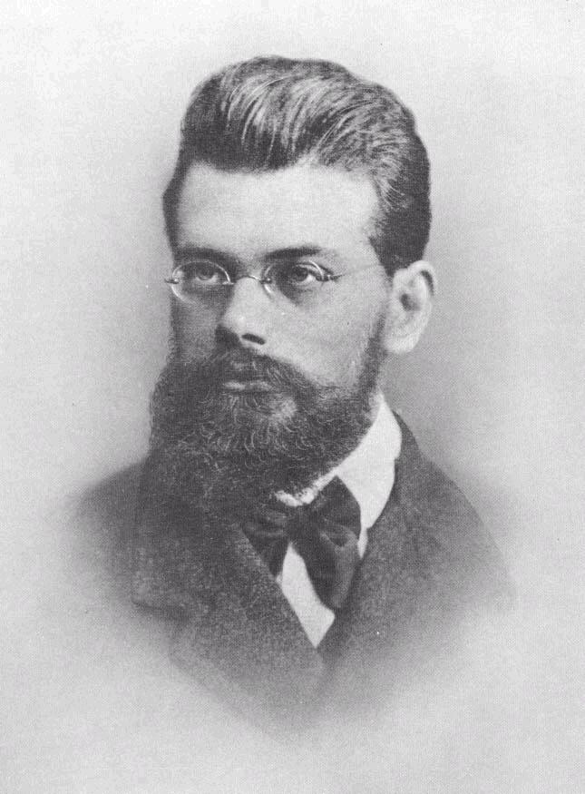
Austrian physicist Ludwig Boltzmann substantially deepened the theory in 1872, deriving the distribution from first principles via his celebrated H-theorem and connecting it to the concept of entropy in statistical mechanics[2]. Boltzmann showed that the Maxwell distribution is the unique equilibrium distribution: any other initial distribution will evolve toward it through molecular collisions, provided the gas is sufficiently dilute (the Stosszahlansatz, or "molecular chaos" assumption).
The combined Maxwell–Boltzmann framework applies to classical ideal gases — dilute collections of point-like particles that interact only through brief elastic collisions[3]. It fails for quantum gases (where Fermi–Dirac or Bose–Einstein statistics apply) and for dense liquids (where intermolecular forces are always present). Within its domain of validity, it is a cornerstone of the kinetic theory of gases, explaining macroscopic properties — pressure, temperature, viscosity, diffusion, and thermal conductivity — from microscopic molecular motion[4].
The 2D version derived here is relevant to surface physics, thin-film adsorption layers, and 2D electron gases, and serves as an excellent pedagogical simplification of the full 3D theory.

Source: Wikimedia Commons
Source: Wikimedia Commons

The Ideal Gas Model
Derivation from First Principles (2D)
For a two-dimensional ideal gas at temperature \(T\), the speed distribution can be derived in four steps using statistical mechanics and coordinate geometry[6]:
-
Independent Gaussian velocity components (Maxwell's postulate):
In thermal equilibrium, the probability density for each velocity component \(v_x\) and \(v_y\) is independent and Gaussian with zero mean. This follows from the Boltzmann factor \(e^{-E/k_BT}\) applied to the kinetic energy \(E = \tfrac{1}{2}m v_x^2\) of each degree of freedom[1]: \[ f(v_x) = \sqrt{\frac{m}{2\pi k_B T}}\exp\!\left(-\frac{m v_x^2}{2k_BT}\right),\qquad f(v_y) = \sqrt{\frac{m}{2\pi k_B T}}\exp\!\left(-\frac{m v_y^2}{2k_BT}\right). \] Independence gives the joint density as the product: \[ f(v_x,v_y) = \frac{m}{2\pi k_BT}\exp\!\left(-\frac{m(v_x^2+v_y^2)}{2k_BT}\right). \] This is already normalised: \(\iint f(v_x,v_y)\,dv_x\,dv_y = 1\). Physically, independence reflects the isotropy of space — there is no preferred direction in an equilibrium gas. -
Polar coordinate transformation — from \((v_x,v_y)\) to \((v,\theta)\):
We seek the marginal distribution of the speed \(v = \sqrt{v_x^2+v_y^2}\). Writing \(v_x = v\cos\theta\) and \(v_y = v\sin\theta\), the Jacobian of the transformation is \[ \left|\frac{\partial(v_x,v_y)}{\partial(v,\theta)}\right| = v, \] so \(dv_x\,dv_y = v\,dv\,d\theta\). Because \(f(v_x,v_y)\) depends only on \(v\) (it is isotropic), integrating over \(\theta\in[0,2\pi)\) gives: \[ f(v)\,dv = \left[\int_0^{2\pi} \frac{m}{2\pi k_BT}\exp\!\left(-\frac{mv^2}{2k_BT}\right) v\,d\theta\right]dv = \frac{m}{k_BT}\,v\,\exp\!\left(-\frac{mv^2}{2k_BT}\right)dv. \] The factor of \(v\) (rather than \(v^2\) as in 3D) arises because the "boundary" of velocity space at radius \(v\) in 2D is a circle (perimeter \(2\pi v\)) rather than a sphere (surface area \(4\pi v^2\)). -
Normalization verification:
Confirming \(\int_0^\infty f(v)\,dv = 1\): \[ \int_0^\infty \frac{m}{k_BT}\,v\,e^{-mv^2/(2k_BT)}\,dv. \] Substituting \(u = mv^2/(2k_BT)\), \(du = (m/k_BT)\,v\,dv\): \[ \int_0^\infty e^{-u}\,du = 1. \quad\checkmark \] -
Key characteristic speeds and equipartition:
The three characteristic speeds follow from moments of \(f(v)\):- Most probable speed (peak of \(f\)): \(\displaystyle v_p = \sqrt{\frac{k_BT}{m}}\)
- Mean speed: \(\displaystyle\langle v\rangle = \int_0^\infty v\,f(v)\,dv = \sqrt{\frac{\pi k_BT}{2m}}\)
- RMS speed: \(\displaystyle v_\text{rms} = \sqrt{\langle v^2\rangle} = \sqrt{\frac{2k_BT}{m}}\)
The equipartition theorem states that each quadratic degree of freedom contributes \(\tfrac{1}{2}k_BT\) to the average energy. In 2D there are two translational degrees of freedom, so \[ \langle KE\rangle = \tfrac{1}{2}m\langle v^2\rangle = \tfrac{1}{2}m\cdot\frac{2k_BT}{m} = k_BT, \] which gives the simulation's temperature estimate: \(T = \langle KE\rangle / k_B\).
This derivation, first completed by Maxwell using purely probabilistic reasoning in 1860, stands as one of the earliest applications of statistics to physics and remains a cornerstone of kinetic theory and statistical mechanics.
References
Simulation: hard-disk 2D molecular dynamics with elastic wall reflections. Spatial hash grid O(N) collision detection. Histogram (green) and running average (red) are compared with the theoretical 2D Maxwell–Boltzmann curve (gray dashed) computed from the instantaneous mean kinetic energy. Units: length in nm, time in ps; 1 sim unit = 1000 m/s.